线性化电阻式传感器电桥的两种技术

时间：2023-04-11

电阻式传感器的电阻取决于物理变量，例如温度或力。这些设备的电阻变化百分比通常很小。例如，应变计电阻在其整个工作范围内的总变化可能小于 1%。

辨别这些小值需要高度的测量电路。桥接电路使我们能够更轻松地执行这些测量。然而，即使我们使用线性传感器，桥式电路的输出也可能与测量的物理变量具有非线性关系。

在这些情况下，我们可以使用软件或硬件技术来消除桥非线性误差。在本文中，我们将了解两种不同的电阻式传感器电桥线性化技术。

电阻传感器的桥接非线性

考虑具有以下线性响应的电阻式压力传感器：

R传感器=R0+Mx $R_{传感器} = R_{0} + M x$

其中 R 0是传感器在零压力下的初始电阻，x 是被测量（压力）的值，M 是传感器响应的斜率。为了简化我们未来的方程式，让我们假设 M 的值等于传感器的初始电阻 (R 0 ) 的值，因此，传感器响应为 $R_{0} (1 + x)$ 。

通常，电阻式传感器的电阻变化百分比很小，我们需要使用电桥电路来更轻松地进行测量。图 1 描绘了该传感器的常见电桥配置。

电阻传感器的常见电桥配置

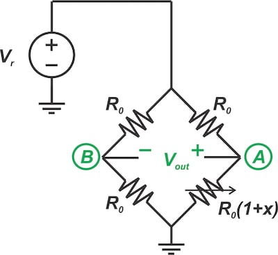
图 1.电阻传感器的常见电桥配置

请注意，电桥的其他三个电阻器的阻值为 R 0。这种桥式电阻器的选择限度地提高了输出 (V out ) 对传感器电阻变化的灵敏度。可以得到输出方程为：

$V_{o u t} = V_{A} ? V_{B} = V_{r} (\frac{R_{0} (1 + x)}{R_{0} + R_{0} (1 + x)} ? \frac{1}{2})$

这简化为：

$V_{o u t} = V_{r} (\frac{x}{2 (2 + x)})$

等式 1。

如您所见，电桥输出与电阻值 (x) 变化之间的关系不是线性的。有了 $x ? 2$ ，我们可以通过以下线性关系近似上述方程：

$V_{o u t} \approx V_{r} (\frac{x}{4})$

等式 2。

图 2 描述了实际情况（公式 1）和理想输出（公式 2）的电桥 $\frac{V_{o u t}}{V_{r}}$ 的归一化输出。

等式 1 和 2 的非线性（蓝色）和理想（红色）输出

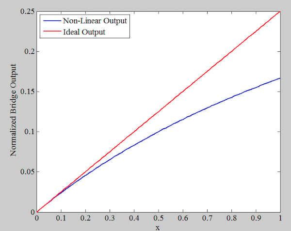
图 2.等式 1 和 2 的非线性（蓝色）和理想（红色）输出

正如预期的那样，与线性响应的偏差随 x 的增加而增加。

会引入多少非线性误差？

让我们量化上述桥式电路的非线性误差。我们可以将等式 1 重写为：

$V_{o u t} = V_{r} (\frac{x}{4}) (\frac{1}{1 + \frac{x}{2}})$

假设 $\frac{x}{2} << 1$ ，我们可以使用泰勒定理得到上述函数的近似值：

$V_{o u t} = V_{r} (\frac{x}{4}) (1 ? \frac{x}{2})$

将此结果与公式 2 进行比较，我们可以计算出误差的大小：

$E_{非线性} = V_{r} (\frac{x}{4}) (\frac{x}{2})$

将其除以公式 2 给出的预期理想值，我们可以获得给定电阻变化 (x) 的终点线性误差百分比：

$百分比误差 = \frac{x}{2} \times 100 %$

计算非线性误差的示例

考虑一个响应为 $R_{s e n s o r} = R_{0} (1 + x)$ 的传感器。假设 $R_{0} = 100 Ω$ 并且 x 在整个工作范围内的值为 0.01。线性误差百分比将为：

$百分比误差 = (\frac{0.01}{2}) \times 100 % = 0.5 %$

请注意，虽然我们可以使用软件来消除传感器线性误差，但线性响应是可取的，因为它可以提高测量精度并便于系统校准。有不同的电路拓扑可用于线性化电桥电路。

在本文的其余部分，我们将研究两种不同的桥接线性化技术。

方法 1：创建与电阻变化 (x) 成正比的电压

我们将在本文中讨论的种线性化技术如图 3 所示。让我们首先研究这种技术的基本思想，然后看看图 3 中的电路如何实现这一思想。

说明电阻传感器电桥模拟线性化的电路

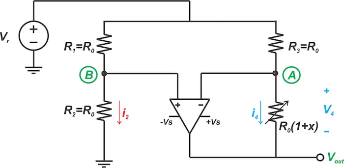
图 3.一种用于线性化电阻传感器电桥的电路

图 4 显示了强制流过我们的线性传感器的固定电流 $I_{R e f}$ 。

强制固定电流 (IRef) 通过线性传感器

图 4.强制通过线性传感器的固定电流 (I Ref )

在这种情况下，传感器两端产生的电压为：

$V_{s e n s o r} = I_{R e f} \times R_{0} (1 + x)$

可以重新排列为：

$V_{s e n s o r} = R_{0} \times I_{R e f} + R_{0} \times I_{R e f} \times x$

项是常数值，而第二项与传感器电阻 (x) 的变化成正比。如果我们可以省略常数项，我们将得到与 x 呈线性关系的电压。

电路实现

图 3 中的电路使用上述思想对桥式电路进行线性化。由于运算放大器输入理想情况下不吸取任何电流，因此节点 B 处的电压将具有恒定值：

$v_{B} = \frac{R_{0}}{R_{0} + R_{0}} V_{r} = \frac{V_{r}}{2}$

负反馈以及运算放大器的高增益将迫使运算放大器的反相和非反相输入具有相同的电压：

$v_{A} = v_{B} = \frac{V_{r}}{2}$

由于R3两端处于恒定电位，因此将有恒定电流流过。换句话说，运算放大器使 R3 充当电流源，迫使 $\frac{V_{r}}{2 R_{0}}$ 的恒定电流进入传感器。因此，传感器两端的电压将为：

$V_{4} = \frac{V_{r}}{2 R_{0}} \times R_{0} (1 + x) = \frac{V_{r}}{2} + \frac{V_{r}}{2} x$

项是应从 Vout 方程中消除的常数值。第二项与传感器电阻变化 (x) 成正比，应出现在输出方程中。应用基尔霍夫电压定律，我们发现 V为：

$V_{o u t} = ? V_{4} + V_{A} = ? (\frac{V_{r}}{2} + \frac{V_{r}}{2} x) + V_{A}$

因此，我们只需要 V A等于 $\frac{V_{r}}{2}$ 。这已经满足了，这导致：

$V_{o u t} = ? \frac{V_{r}}{2} x$

因此，输出与x具有线性关系。

方法 2：创建与电阻变化 (x) 成比例的电流

我们将在本文中讨论的第二种桥接线性化技术如图 5 所示。

说明电阻传感器电桥模拟线性化的电路

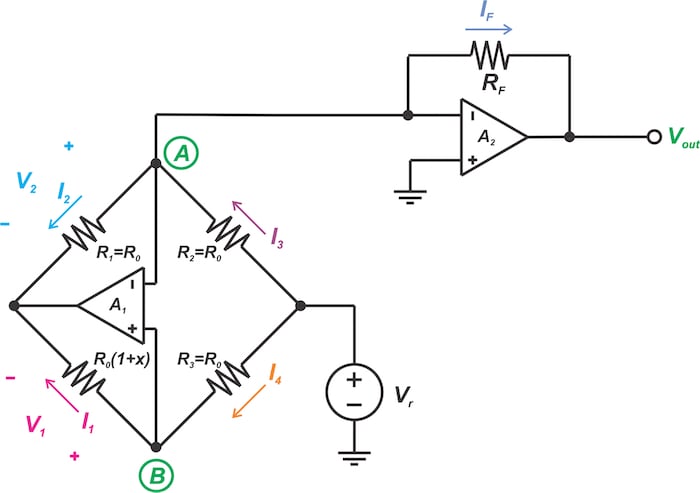
图 5.电阻传感器电桥模拟线性化的另一个电路

让我们再次看一下这种技术的基本思想，然后检查其电路实现。

图 6 说明了第二种线性化技术。

线性化技术迫使通过电路分支的电流与传感器的电阻成正比

图 6.强制电流通过电路分支的线性化技术与传感器的电阻成正比

它迫使通过电路分支（分支 1）的电流与传感器电阻成正比：

$I_{1} = I_{R e f} \times R_{0} (1 + x)$

其中 I Ref是一个常数值。然后，它执行当前域减法以消除常数项 $I_{R e f} \times R_{0}$ 。为此，通过分支 2 的电流设置为 $I_{R e f} \times R_{0}$ 。因此，通过分支 3 的电流将为 $I_{R e f} \times R_{0} x$ —与传感器电阻 (x) 的变化成正比。

电路实现

让我们看看图 5 中的电路是如何实现上述想法的。同样，负反馈和运算放大器的高增益将迫使两个运算放大器（A 1 和A 2 ）的反相和非反相输入具有相同的电压：

$v_{A} = v_{B} = 0$

等式 3。

因此，我们有V 1 = V 2这导致

$R_{0} (1 + x) \times I_{1} = R_{0} \times I_{2}$

这简化为：

$I_{2} = I_{1} + I_{1} \乘以 x$

等式 4。

我们知道I 1 = I 4并且考虑到等式 3，我们有：

$I_{1} = I_{4} = \frac{V_{r} ? v_{A}}{R_{0}} = \frac{V_{r}}{R_{0}}$

将其代入等式 4，我们得到：

$I_{2} = \frac{V_{r}}{R_{0}} + \frac{V_{r}}{R_{0}} \times x$

因此，I 2是常数值和与x成正比的项之和。我们只需要利用基尔霍夫电流定律消去输出电流方程中的常数项即可。通过 R2 的电流为节点 A 提供等于 $\frac{V_{r}}{R_{0}}$ 的电流，导致：

$I_{F} = ? \frac{V_{r}}{R_{0}} \times x$

因此，我们得到：

$V_{o u t} = V_{r} \times \frac{R_{F}}{R_{0}} \times x$

与种技术相比，图 5 中的电路需要一个额外的运算放大器。然而，对于这两种运算放大器解决方案，我们可以通过选择 \[\frac{R_F}{R_0}\] 比率来任意设置增益。

上一篇：MOS管漏电流的6大原因

下一篇：良好通信链路性能的要求：IQ 调制和解调